My Mathematical Journey: From F = ma to E = mc^2
By: David Bressoud @dbressoud

David Bressoud is DeWitt Wallace Professor Emeritus at Macalester College and former Director of the Conference Board of the Mathematical Sciences
This month I have chosen to write about the genesis of a very important book in my development as a writer, Second Year Calculus: From Celestial Mechanics to Special Relativity. The title is misleading. This is really a textbook for vector calculus, not the traditional multi-variable calculus course usually taught in the second year of college calculus. I wanted to title it From F = ma to E = mc^2, but my editor at Springer told me that book titles could not include equations because those could not be alphabetized. Furthermore, as a textbook, potential adopters needed to know for which course it would be appropriate. A few years later Herb Wilf and Doron Zeilberger published their book entitled A = B, and my book has never found a market among courses in second year calculus. But I was stuck with the title.
I am very proud of this book. Published in 1991, it has gone through many printings and still manages decent sales. I continue to hear from grateful readers who recently discovered it, thanking me for showing why the calculus they studied many years ago is actually useful.
Problem: Show how Newton’s equation F = ma leads to Einstein’s conclusion that E = mc^2
This is the problem that provides the backbone, the intellectual need, for this book. But I am getting ahead of myself. How I came to write this book and what I intended to accomplish is a long story.

Figure 1: Harold (Ed) Edwards (1936–2020)
For the spring term of 1987 the State College Area High School was faced with an unprecedented problem. Seven of their students had completed BC Calculus in their junior year and wanted to study several variable calculus. The high school felt that they would be best served by a class just for them taught by a member of the Penn State mathematics faculty. Rich Herman, who was then Chair of the department, asked if I would take it on. I agreed.
My own relationship with several variable calculus had been rocky. I had studied calculus in high school and taken the AP Calculus exam in the spring of 1968. That was the last year before the course was split into AB and BC Calculus. There was only one exam, covering the entire year of college-level single variable calculus. At Swarthmore, where I matriculated that fall, one semester of calculus credit was awarded for a 3 or 4, a full year for a 5. I had earned a 5, which put me into several variable calculus in my freshman year.
Jim England, then a new faculty member, chose the second volume of Tom Apostol’s Calculus as the text. I was totally overwhelmed, and it put me off analysis. Swarthmore had very flexible requirements for the mathematics major, and I subsequently managed to avoid taking either real or complex analysis as an undergraduate. I did, however, study point-set topology with Michael Gemignani’s Elementary Topology as our text, a book with which I fell in love. It was my first extended exposure to mathematics as puzzle-solving.
In graduate school, I eagerly signed up for Differential Topology, naively expecting it would simply build on what I had already learned. I do not know if it was the textbook, the instructor, or where I was at the time, but I was totally mystified by everything that was presented in this course. I never could figure out what differentials actually were or why they behaved as they did. I did manage to master their manipulation and the use of short exact sequences, and I succeeded in the course. But it put me off topology.
Back to my seven students at the State College Area High School. I knew I was facing very talented scholars. Most of them would go on to earn doctorates and hold prestigious positions. Marguerite Eisenstein, one of the two women in the class, later earned a PhD at Brandeis under the direction of a close colleague, Ira Gessel. I decided that this would be an opportunity to close gaps in my own educational experience by focusing the course as Apostol had done, on vector calculus.
As I searched the library for an appropriate text, I came across Harold Edwards’ Advanced Calculus: A Differential Forms Approach. It seemed perfect. It was certainly challenging. It finally explained for me what differentials really are and why they act as they do (see also my September, 2021 Launchings column), and it ended on the high note of explaining special relativity and the derivation of Einstein’s famous equation, E = mc^2. Edwards’ text was my first experience with the use of the history of mathematics to provide framing and motivation when teaching mathematics. Over the years, I would come to appreciate his insightful accounts of the development of several important mathematical advances. All of his books are gems.
I cannot say that using Edwards’ text was a success. My students generally had the same experience I had known with Apostol’s Calculus, vol II. They were more confused than enlightened by all of the unfamiliar concepts suddenly coming at them. Marguerite later told me that she did appreciate learning at that stage of her career that you do not always need to understand everything presented to you in a given course. Sometimes you can just let the mathematics wash over you, knowing that it is there if you ever need to go back and really learn it.
But I was still enchanted by the approach that Edwards had taken. I decided to rework his material into a textbook that could be used with capable undergraduates. Over the fall semesters of 1989 and 1990 I presented a course based on my own reworking of Advanced Calculus to students taking several variable calculus within Penn State’s honors program.
I added an additional twist. Around that time, Subrahmanyan Chandrasekhar (1910–1995) had visited Penn State and given a series of lectures on his latest passion, Newton’s Mathematical Principles of Natural Philosophy. My eyes were opened to the beauty and importance of this book. Chandrasekhar showed me that I could dare to try to read it for myself, which I did with delight. Not cover-to-cover, but I worked through the early material and dipped in to sample its further delights. My own manuscript began to take shape as I conceived of a progression that would start with Newton’s Principia, build through the use of differential forms to compute the work done by a force field or the flux through a surface created by a known flow, crescendo with the applications to the mathematics of electricity and magnetism, and end with Einstein’s special relativity. That was the course I taught and the book I created.
I have much more to say about this book and how I would continue to be inspired by the Principia throughout my career, but for now I want to close by explaining how F = ma leads to E = mc^2.
Newton did not actually say that force equals mass times acceleration. He said that force equals the rate of change with respect to time of momentum, mass times velocity. If one assumes that mass is invariant, then this is equivalent to mass times acceleration. But Maxwell’s equations had led late 19th century physicists to question the invariance of mass at high velocity.
Maxwell’s equations, the differential equations governing the interactions of electricity and magnetism, are usually taught as four equations. Two are vector equations, and two are scalar equations. Because time is an important variable in these equations, it is more appropriate to think of them as equations in 4-dimensional space-time, reducing them to two equations in four dimensions. (This is a slight oversimplification. The most effective representations are as identities for the differentials of two-forms in four-dimensional space. See page 345 in Second Year Calculus.) The vector equations occur in the spatial dimensions, and the scalar equations are placed in the time dimension. Now something interesting happens, these two equations are natural duals of each other, obtained by switching the electric and magnetic fields.
Maxwell went on to push this a bit further. Gravitational force is described by a vector field, showing the direction and magnitude of gravitational attraction at any point. In the late 1700s, Laplace realized that much of the work in celestial mechanics, explaining the movement of celestial bodies, could be simplified by working instead with gravitational potential, essentially the potential energy at any point. This has the advantage that one is working with scalars rather than vectors.

Figure 2: d’Alembert’s differential equation for a vibrating string and the differential equation satisfied by each component of the electromagnetic potential.
Maxwell had the audacity to wonder whether his four-dimensional description of electro-magnetism also possessed a potential. He found that it did. Unlike gravitational potential, electro-magnetic potential has four dimensions. Then came the surprise. In each dimension, the component of the electro-magnetic potential satisfies a four-dimensional analog of the differential equation, known as the d’Alembertian (Figure 2), that governs the vibrations of a string. As is well-known, plucking a very long string sets up waves that will travel out from the disturbance at a speed that is determined by the properties of the string. Maxwell’s four-dimensional d’Alembertian suggests that any disturbance in the electro-magnetic potential will propagate out in all directions at a speed determine by the electrical and magnetic properties of the space in which the disturbance occurs. Measuring these properties as accurately as he could, Maxwell discovered that the speed of propagation, denoted by c, agreed with the then known speed of light, about 300,000 kilometers per second.
This prompted some outrageous speculation. If this was really happening, then it might be possible to engineer a precise disturbance in the electro-magnetic potential that would spread out in all directions at the speed of light and, perhaps, could be detected at some distance from the source. One might be able to create instantaneous communication across considerable distances, perhaps even kilometers of separation, without any physical connection.
The scientific community was highly skeptical. After all, gravitational potential is a useful fiction, but no one would claim that it had any tangible reality. Maxwell died in 1879 with his speculation still just that, but eight years later Heinrich Rudolf Hertz built an apparatus capable of detecting electro-magnetic waves. Within a few years Guglielmo Marconi and Alexander Popov had each figured out how to use this to send morse code wirelessly at the speed of light. Today electro-magnetic waves are more commonly known as radio waves. It is hard to imagine what our world would be like if the existence of these waves had remained hidden. They provide the physical reality that enables everything from cell phones to garage door openers to global positioning. Their existence was only revealed by the differential equation that electro-magnetic potential was discovered to satisfy.

Figure 3: The contraction factor of an object traveling at velocity v relative to the original observer.
Another surprise was in store. Among Newton’s assumptions at the foundation of his Principia was the statement that all motion is relative, that there is no way to physically distinguish between a body at rest and body moving at a constant velocity. The laws of physics must be the same for both. But in the 1890s both the Irish physicist George Francis Fitzgerald and the Dutch physicist Hendrick Antoon Lorentz realized that Maxwell’s electromagnetic potential was not left invariant under natural assumptions about the effect of systems moving at different velocities. They discovered that the laws governing electro-magnetic potential would only remain invariant if distances contract by a factor dependent on the ratio of the velocity to the speed of light (Figure 3).

Figure 4: The Lorentz transformation when shifting to a frame traveling at speed v in the positive x-direction with respect to a initial observer.
Lorentz formulated the linear transformation needed to convert from one observer to a second who is traveling at velocity v in the positive x-direction. An object that appears stationary to the first observer will appear to be moving at speed v in the negative x-direction to the second observer, but with distances contracted by the factor beta as shown in Figure 4. Time itself also contracts.
The contractions are tiny unless one is traveling very close to c, the speed of light. A rocket ship traveling at a million kilometers per hour would experience contractions of 0.99999957, less than one part in two million. Nevertheless, the contractions are real enough that global positioning satellites traveling at a mere 15,000 km/hr must take them into account.
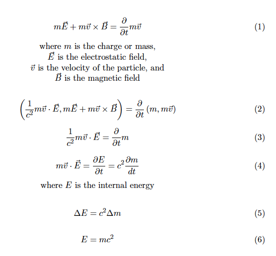
Figure 5: Derivation of Einstein’s equation.
The scene has been set to derive Einstein’s equation. At this point I need to switch to some technical mathematics for which the justifications can be found in Section 11.5 of Second Year Calculus. The electromagnetic force acting on a charged particle is given by the left side of equation (1) in Figure 5. The right side is simply the rate of change of the momentum of the particle. But there are also time components to both force and momentum that are determined by the need for invariance under the Lorentz transformation, as expressed in equation (2). In equation (3) we pull out the equality of the time components and see that a change in velocity also implies a change in mass, although the coefficient of c^2 indicates how extremely small this would be.
The left side of equation (3) is momentum multiplied by the strength of the electrostatic field which is the rate of change of energy, producing equations (4) and (5), which establishes the connection between mass and energy. Under the assumption that no mass corresponds to no energy, we conclude that that the total energy is the square of the speed of light multiplied by the mass, equation (6).
In his Gibbs lecture of 1972, “Missed Opportunities,” Freeman Dyson used the derivation of Einstein’s equation as one of his illustrations of how mathematicians ignore the work of physicists to their detriment. Three years after Einstein published his results on Special Relativity, Hermann Minkowski pointed out that the mathematical basis of Einstein’s discovery lay in replacing the Galilei group, the group of transformations that assume the invariance of time and distance and under which Newtonian physics operates, with the Lorentz group, which includes the Lorentz transformations. This simple observation is all that is required for the derivation of Einstein’s equation.
As Dyson points out, the leading mathematicians of the 1860s and ‘70s—when Maxwell’s equations were disseminated—were perfectly capable of realizing that these equations required invariance under these more complex transformations, but they were paying little or no attention to what was happening in physics. A missed opportunity.
I am pleased to say that the situation has improved considerably, not least because of the efforts of Freeman Dyson and others like him who straddled the worlds of mathematics and physics. Today there is a great deal of cross-fertilization, some of which I will explain in later columns.
Download the list of all past Launchings columns, dating back to 2005, with links to each column.